
A/B Testing Python Project: Testing whether a Smart Ad increases consumer response rates
1) Problem Scenario
As part of its operations, a business shows its customers an ad, the purpose of which is to encourage the customer to fill out a ‘BIO questionnaire’. Customers may see this questionnaire and choose to either:
- fill it out with the option of clicking on ‘Yes’
- reject filling it out with the option of clicking ‘No’
- Ignore the questionnaire entirely by clicking neither ‘Yes’ or ‘No’
The ad the business is currently using is called a ‘dummy ad’; it is plain and not interactive. The response rate is a measure of effectiveness of the ad, and is equal to the number of ‘Yes’ or ‘No’ responses collectively divided by the total number of customers the ad is shown to.
The business wants to come up with a new ad that increases this response rate. It calls this the ‘Smart Ad’ or the ‘Creative Ad’, an interactive, colourful cousin of its blander counterpart. It wishes to see whether or not showing this Smart Ad to customers will actually increase the response rate
1.2) Business Objective and Effect Size
The company aims to see a minimum detectable effect of a 2% increase in response rates as a result of the new Creative Ad
1.3) The question we want to answer and our hypotheses:
“Is there a statistically significant difference in response rates to the BIO questionnaire between the control and exposed groups?”
We will see shortly that in the column descriptions, the description of the auction_id column says that:
“The user may see the BIO questionnaire but choose not to respond. In that case both the yes and no columns are zero.”
In this context, we are not trying to find out which group saw more people choose ‘Yes’ and fill out the questionnaire. We are simply finding which group elicited more people to respond, whether their response was ‘Yes’ or ‘No’
So, to create our outcome variable, we need to find out the proportions of respondents (either ‘yes’ = 1 or ‘no’ = 1) to the total number of people, for both the control and exposed groups
1.31) Null and Alternative Hypotheses
We hypothesise that our ‘exposed’ group will have a higher response rate compared to our ‘control’ group. So we will conduct a one-tailed test.
If pc is the response rate of the control group and pe is the response rate of the exposed group, then:
H0: SmartAd recipients that receive the Creative Ad will have the same response rate as the response rate of recipients who receive the dummy ad
pc = pe
H1: SmartAd recipients that receive the Creative Ad will have a higher response rate than the response rate of recipients who receive the dummy ad
pc < pe
1.4) Limitations
These primarily result from the existence of other independent variables we do not account for, as they might have effects on the outcome. For example, the day of the week or hour of the day that the creative ad is shown to individuals might influence whether or not they respond to it.
One way to deal with this is to fix these values. This would mean, for example, we only use those observations from the dataset where the date or hour value is the same. That is to say, we may only look at those individuals who saw the creative ad on the same day or even within the same hour.
However, this will lead to a substantial reduction in sample size, which will directly and negatively impact our hypothesis testing. Therefore, we do not use this approach.
Another way to minimise these effects is to have truly random sampling. This is done to a. Distribute co-variates evenly and b. eliminate statistical bias as much as possible.
Since we did not sample this data ourselves, we cannot be 100% certain about the randomness of the sampling
1.5) Data Source
The dataset is obtained from Kaggle and was uploaded by user Osuolale Emmanuel
2) Loading and Pre-Processing Data
# imports

import pandas as pd
import numpy as np
import matplotlib.pyplot as plt
import matplotlib.style as style
import seaborn as sns

%matplotlib inline

# visualisation presets

style.use('fivethirtyeight')
preferred_font = {'fontname':'Helvetica'}
# read in data

data = pd.read_csv('/Users/alitaimurshabbir/Desktop/AdSmartABdata - AdSmartABdata.csv')
print('size of dataset: {0} and number of columns: {1}'.format(len(data), len(data.columns)))

# data types

print('------------')
print('column types:')

for column, dtype in data.dtypes.iteritems():
    print(column, dtype)
size of dataset: 8077 and number of columns: 9
------------
column types:
auction_id object
experiment object
date object
hour int64
device_make object
platform_os int64
browser object
yes int64
no int64
2.1) Description of Columns
| Column | Description |
|---|---|
| auction_id | the unique id of the online user who has been presented the BIO. In standard terminologies this is called an impression id. The user may see the BIO questionnaire but choose not to respond. In that case both the yes and no columns are zero |
| experiment | which group the user belongs to - control or exposed. |
| date | the date in YYYY-MM-DD format |
| hour | the hour of the day in HH format. |
| device_make | the name of the type of device the user has e.g. Samsung |
| platform_os | the id of the OS the user has. |
| browser | the name of the browser the user uses to see the BIO questionnaire. |
| yes | 1 if the user chooses the “Yes” radio button for the BIO questionnaire. |
| no | 1 if the user chooses the “No” radio button for the BIO questionnaire. |
2.2) Check for duplicates and null values
data[data.duplicated(['auction_id'], keep=False)]
| auction_id | experiment | date | hour | device_make | platform_os | browser | yes | no |
|---|
There are no duplicates
data.isnull().sum().sum()
0
There are no null values
2.3) Get data in the required format
# create outcome variable 'response'. If either 'yes' or 'no' = 1, then response = 1
# if both 'yes' and 'no' = 0, then response = 0

conditions = [
    (data['yes'] == 0) & (data['no'] == 0),
    (data['yes'] == 1) & (data['no'] == 0),
    (data['yes'] == 0) & (data['no'] == 1),
]

outputs = [0, 1, 1]

data['response'] = np.select(conditions, outputs, 99)
# create a crosstab to understand relevant variables

# responders in control group
control = data[data['experiment'] == 'control']['response']

# responders in exposed group
exposed = data[data['experiment'] == 'exposed']['response']

cross_tab = pd.DataFrame(pd.crosstab(data['experiment'], data['response']))

# add response rate for each group
cross_tab['response_rate'] = cross_tab[1]/(cross_tab[0] + cross_tab[1])
# create dataframes that hold data for either group, then concatenate

control_sample = data[data['experiment'] == 'control']

exposed_sample = data[data['experiment'] == 'exposed']

ab_test = pd.concat([control_sample, exposed_sample], axis = 0)

ab_test
| auction_id | experiment | date | hour | device_make | platform_os | browser | yes | no | response | |
|---|---|---|---|---|---|---|---|---|---|---|
| 3 | 00187412-2932-4542-a8ef-3633901c98d9 | control | 2020-07-03 | 15 | Samsung SM-A705FN | 6 | 0 | 0 | 0 | |
| 4 | 001a7785-d3fe-4e11-a344-c8735acacc2c | control | 2020-07-03 | 15 | Generic Smartphone | 6 | Chrome Mobile | 0 | 0 | 0 |
| 5 | 0027ce48-d3c6-4935-bb12-dfb5d5627857 | control | 2020-07-03 | 15 | Samsung SM-G960F | 6 | 0 | 0 | 0 | |
| 6 | 002e308b-1a07-49d6-8560-0fbcdcd71e4b | control | 2020-07-03 | 15 | Generic Smartphone | 6 | Chrome Mobile | 0 | 0 | 0 |
| 7 | 00393fb9-ca32-40c0-bfcb-1bd83f319820 | control | 2020-07-09 | 5 | Samsung SM-G973F | 6 | 0 | 0 | 0 | |
| ... | ... | ... | ... | ... | ... | ... | ... | ... | ... | ... |
| 8065 | ffbc02cb-628a-4de5-87fc-5d76b7d796e5 | exposed | 2020-07-09 | 17 | Generic Smartphone | 6 | Chrome Mobile | 0 | 0 | 0 |
| 8067 | ffc594ef-756c-4d24-a310-0d8eb4e11eb7 | exposed | 2020-07-05 | 1 | Samsung SM-G950F | 6 | Chrome Mobile WebView | 0 | 0 | 0 |
| 8071 | ffdfdc09-48c7-4bfb-80f8-ec1eb633602b | exposed | 2020-07-03 | 4 | Generic Smartphone | 6 | Chrome Mobile | 0 | 1 | 1 |
| 8072 | ffea24ec-cec1-43fb-b1d1-8f93828c2be2 | exposed | 2020-07-05 | 7 | Generic Smartphone | 6 | Chrome Mobile | 0 | 0 | 0 |
| 8075 | ffeeed62-3f7c-4a6e-8ba7-95d303d40969 | exposed | 2020-07-05 | 15 | Samsung SM-A515F | 6 | Samsung Internet | 0 | 0 | 0 |
8077 rows × 10 columns
# find standard deviation for each group and display crosstab

std_deviation = ab_test.groupby('experiment')['response'].std()
cross_tab = pd.concat([cross_tab, std_deviation], axis = 1)
cross_tab.rename({'response':'std_deviation'}, axis = 1, inplace = True)
cross_tab
| 0 | 1 | response_rate | std_deviation | |
|---|---|---|---|---|
| experiment | ||||
| control | 3485 | 586 | 0.143945 | 0.351077 |
| exposed | 3349 | 657 | 0.164004 | 0.370325 |
-
It seems that the response rate for the exposed group is about 2% greater than in the control group, which is what we expected to see
-
Standard deviation across both groups is also very similar
3) EDA
3.1) Number of Observations in Each Sample
colours = ['#564787', '#F2FDFF']
experiment_countValues = ab_test['experiment'].value_counts()
experiment_countValues.plot(kind = 'pie', colors = colours, figsize = (6, 6),
            title = 'Sizes of Control and Exposed Groups - % of Total Observsations',
            fontsize = 13, autopct='%1.1f%%', shadow = True)
<AxesSubplot:title={'center':'Sizes of Control and Exposed Groups - % of Total Observsations'}, ylabel='experiment'>
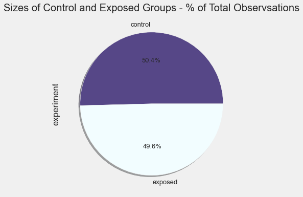
- There is thankfully an equal split of observations in our control and exposed groups
3.2) Response Rates of Both Groups
plot = pd.DataFrame(ab_test.groupby('experiment')['response'].mean()).reset_index()
plt.figure(figsize = (6, 6))
plt.bar(plot['experiment'], plot['response'], color = 'slateblue')
plt.title('Overall Response Rates of control vs exposed group', **preferred_font, fontsize = 16)
plt.xlabel('Group', **preferred_font, fontsize = 12)
plt.ylabel('Response Rate', **preferred_font, fontsize = 12)
Text(0, 0.5, 'Response Rate')
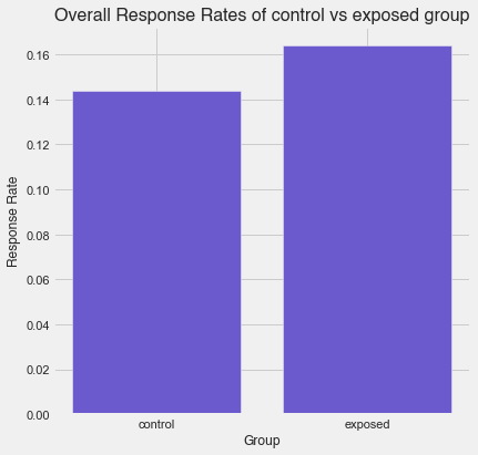
- As shown in the crosstab previously, the exposed group has about a 2% higher response rate
3.3) Number of Responses By Time of Day
plt.figure(figsize = (8, 4))
plt.bar(ab_test.groupby('hour')['response'].sum().index,
        ab_test.groupby('hour')['response'].sum(), color = '#9AD4D6')
plt.title('Number of Responses by Hour - both groups combined', **preferred_font, fontsize = 16)
plt.xlabel('Hour of Day', **preferred_font, fontsize = 12)
plt.ylabel('Number of Responses', **preferred_font, fontsize = 12)
Text(0, 0.5, 'Number of Responses')
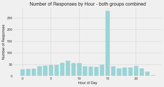
-
The data is dominated for both groups by the time slot of 3 pm. In other words, customers in both the control and exposed groups responded to the dummy and Creative Ad respectively to a much greater extent when they saw the ad at 3 pm.
-
This may simply be because most people check their computers/phones at around this hour, perhaps just before their lunch break finishes. However, this is purely theoretical on my part
3.4) Total Number of Individuals Who Received Either Ad
plt.figure(figsize = (8, 4))
plt.bar(ab_test.groupby('hour')['auction_id'].count().index,
        ab_test.groupby('hour')['auction_id'].count(), color = 'slateblue')
plt.title('Total Number of Individuals Who Received an Ad, by Hour - both groups combined',
          **preferred_font, fontsize = 14)
plt.xlabel('Hour of Day', **preferred_font, fontsize = 11)
plt.ylabel('Number of Individuals', **preferred_font, fontsize = 11)
Text(0, 0.5, 'Number of Individuals')
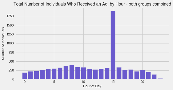
- We see the same phenomenon as above, only this time for all ads received, whether they were responded to or not
3.5) Response Rates by Date and Group
# sort dataframe by date and make a copy

ab_test_date_sorted = ab_test.sort_values(by = ['experiment', 'date'])

# Draw a grouped barplot by date and group

sns.catplot(data = ab_test_date_sorted, kind = "bar", x="date",
            y = "response", hue = "experiment", palette="mako",
            alpha = 0.9, ci = None, aspect = 18/9)

plt.title('Response Rates by Date and Group', size = 18)
Text(0.5, 1.0, 'Response Rates by Date and Group')
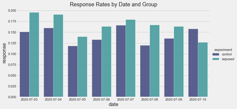
-
The response rate for the exposed group is greater for all days except for the very last date in the experiment.
-
This is interesting as it could point to the existence of a ‘novelty effect’; perhaps customers are only responding to the Creative Ad (exposed group) to a greater extent compared to the dummy ad (control group) simply because the Creative Ad is ‘new’
4) Hypothesis Testing
4.1) What test should we use?
Given that we are working with proportions, 2 samples and a fairly large sample size (n > 4000 for either group), we will use a Z-test for proportions
4.2) Conduct the test
Reiterating our hypotheses:
H0: SmartAd recipients that receive the Creative Ad will have the same response rate as the response rate of recipients who receive the dummy ad
pc = pe
H1: SmartAd recipients that receive the Creative Ad will have a higher response rate than the response rate of recipients who receive the dummy ad
pc < pe
from statsmodels.stats.proportion import proportions_ztest, proportion_confint

# initialise responses for either group into separate variables

control_results = ab_test[ab_test['experiment'] == 'control']['response']
exposed_results = ab_test[ab_test['experiment'] == 'exposed']['response']

# find the number of observations for each group/sample

control_n = control_results.count()
exposed_n = exposed_results.count()

# find the number of successes for each group/sample

successes = [control_results.sum(), exposed_results.sum()]

n_observations = [control_n, exposed_n]

# conduct the test

z_stat, p_val = proportions_ztest(successes, nobs = n_observations)

(lower_con, lower_treat),(upper_con, upper_treat) = proportion_confint(successes,
                                                                       nobs = n_observations,
                                                                       alpha=0.05)
print('z-statistic: {}'.format(z_stat))
print('p-value: {}'.format(p_val))
print(f'95% Confidence Interval for control group: [{lower_con:.3f}, {upper_con:.3f}]')
print(f'95% Confidence Interval for exposed group: [{lower_treat:.3f}, {upper_treat:.3f}]')
z-statistic: -2.4978575502090976
p-value: 0.012494639102152035
95% Confidence Interval for control group: [0.133, 0.155]
95% Confidence Interval for exposed group: [0.153, 0.175]
4.3) Test and Business Conclusions
-
We see that our p-value < 0.05. Therefore, we can reject the null hypothesis. It is highly likely that the response rate of the exposed group which sees the creative ad is greater than the response rate of the control group which sees the dummy ad.
-
Moreover, the confidence intervals tell us a similar story. The CI for the exposed group i) does not include the control group response rate of 0.143945 and ii) does include the 2% increase the business aimed to see (0.143945 + 0.02 = 0.163945)
-
This means that the business can be highly confident that the Creative Ad elicits more response rates from its customers, and that it should from now on show the Creative Ad to all of its customers (the population)