A client, the Category Manager for a supermarket chain, wants to better understand the types of customers who purchase Chips and their purchasing behaviour within the region. The insights from this analysis will feed into the supermarket’s strategic plan for the chip category in the next half year.
The client is particularly interested in customer segments and their chip purchasing behaviour. For example, they require insights on who spends on chips and what drives spends for each customer segment
I need to present a strategic recommendation to my team lead that is supported by data which she can then use for the upcoming category review.
# change "DATE" column to datetime and PROD_NAME to string
df_trans['DATE']=pd.to_datetime(df_trans['DATE'])df_trans['PROD_NAME']=df_trans['PROD_NAME'].astype('string')
# look at distributions and extreme values

df_trans.describe()
STORE_NBR
LYLTY_CARD_NBR
TXN_ID
PROD_NBR
PROD_QTY
TOT_SALES
count
264836.00000
2.648360e+05
2.648360e+05
264836.000000
264836.000000
264836.000000
mean
135.08011
1.355495e+05
1.351583e+05
56.583157
1.907309
7.304200
std
76.78418
8.057998e+04
7.813303e+04
32.826638
0.643654
3.083226
min
1.00000
1.000000e+03
1.000000e+00
1.000000
1.000000
1.500000
25%
70.00000
7.002100e+04
6.760150e+04
28.000000
2.000000
5.400000
50%
130.00000
1.303575e+05
1.351375e+05
56.000000
2.000000
7.400000
75%
203.00000
2.030942e+05
2.027012e+05
85.000000
2.000000
9.200000
max
272.00000
2.373711e+06
2.415841e+06
114.000000
200.000000
650.000000
Let’s investigate the highest TOT_SALES value
df_trans[df_trans['TOT_SALES']==650]
DATE
STORE_NBR
LYLTY_CARD_NBR
TXN_ID
PROD_NBR
PROD_NAME
PROD_QTY
TOT_SALES
69762
2018-08-19
226
226000
226201
4
Dorito Corn Chp Supreme 380g
200
650.0
69763
2019-05-20
226
226000
226210
4
Dorito Corn Chp Supreme 380g
200
650.0
Since the second highest TOT_SALES value is 29.5, this is clearly an outlier so I will drop this value
df_trans.drop([69762,69763],axis=0,inplace=True)
# Check for duplicate values

df_trans[df_trans.duplicated()]
DATE
STORE_NBR
LYLTY_CARD_NBR
TXN_ID
PROD_NBR
PROD_NAME
PROD_QTY
TOT_SALES
124845
2018-01-10
107
107024
108462
45
Smiths Thinly Cut Roast Chicken 175g
2
6.0
There seems to be a single duplicated row. I will drop this.
df_trans.drop(124845,axis=0,inplace=True)
# clean up PROD_NAME column by
# fixing spaces
foriinrange(25):df_trans['PROD_NAME']=df_trans['PROD_NAME'].replace(i*' ',' ')# removing whitespace
df_trans['PROD_NAME']=df_trans['PROD_NAME'].str.strip()# correcting misspelling of Doritos brand
df_trans['PROD_NAME']=df_trans['PROD_NAME'].str.replace('Dorito','Doritos')df_trans['PROD_NAME']=df_trans['PROD_NAME'].str.replace('Doritoss','Doritos')
df_trans['PROD_NAME'].value_counts().to_frame()
PROD_NAME
Kettle Mozzarella Basil & Pesto 175g
3304
Kettle Tortilla ChpsHny&Jlpno Chili 150g
3296
Cobs Popd Swt/Chlli &Sr/Cream Chips 110g
3269
Tyrrells Crisps Ched & Chives 165g
3268
Cobs Popd Sea Salt Chips 110g
3265
...
...
RRD Pc Sea Salt 165g
1431
Woolworths Medium Salsa 300g
1430
NCC Sour Cream & Garden Chives 175g
1419
French Fries Potato Chips 175g
1418
WW Crinkle Cut Original 175g
1410
114 rows × 1 columns
3.2) Behaviours dataset
# look at data types
df_behv.dtypes# change "LIFESTAGE" and "PREMIUM_CUSTOMER" variables to 'string' type
df_behv['LIFESTAGE']=df_behv['LIFESTAGE'].astype('string')df_behv['PREMIUM_CUSTOMER']=df_behv['PREMIUM_CUSTOMER'].astype('string')
# check for duplicates

df_behv[df_behv.duplicated()]
LYLTY_CARD_NBR
LIFESTAGE
PREMIUM_CUSTOMER
There are no duplicates
4) Data Engineering
# create feature to capture 'packet size'
df_trans['Packet Size']=df_trans['PROD_NAME'].astype('str').str.extractall('(\d+)').unstack().fillna('').sum(axis=1).astype(int)# create feature to capture year and month
df_trans['year_month']=df_trans['DATE'].dt.to_period('M')# create brand name feature
df_trans['brand_name']=df_trans['PROD_NAME'].str.split(' ').str[0]
We can find purchase frequency by looking at the number of transactions segmented by different variables
Code
defuni_plot(feature,color,suptitle,title):a=merged_df[feature].value_counts().to_frame()a.reset_index(inplace=True)a.rename({'index':str(feature),str(feature):'Frequency'},axis=1,inplace=True)a.sort_values(by='Frequency',ascending=True,inplace=True)iflen(a)>10:a=a.iloc[len(a)-10:len(a)]ifmerged_df[feature].dtype==int:merged_df[feature]=merged_df[feature].astype('string')plt.figure(figsize=(10,6))plt.barh(a[feature],a['Frequency'],color=color,alpha=0.7)plt.xlabel('Number of Transactions',size=11)plt.xticks(size=9)plt.ylabel(str(feature),size=11)plt.yticks(size=9)plt.title(title,size=14)plt.suptitle(suptitle)plt.show()
6.11) Lifestage
Code
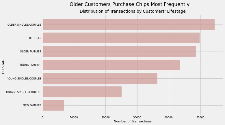
uni_plot('LIFESTAGE','#CF9893','Older Customers Purchase Chips Most Frequently','Distribution of Transactions by Customers\' Lifestage')
# let's also quickly find out how many customers are in each stage
merged_df.LYLTY_CARD_NBR.nunique()# yields 72636
72636
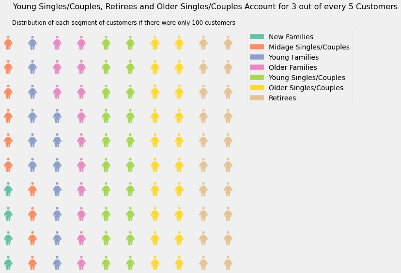
And what proportion of the total customers do customers from the above segment make up?
Code
# and what proportion of the total customers do customers from the above segments
frompywaffleimportWafflecust_count=[]lifestages=list(set(merged_df.LIFESTAGE))foriinlifestages:cust_count.append(merged_df[merged_df['LIFESTAGE']==i]['LYLTY_CARD_NBR'].nunique())cust_per_lifestage=pd.DataFrame({'Lifestage':lifestages,'num_customers':cust_count})value={'New Families':2549,'Young Families':9178,'Midage Singles/Couples':7275,'Retirees':14805,'Older Families':9779,'Young Singles/Couples':14441,'Older Singles/Couples':14609}value=dict(sorted(value.items(),key=lambdax:x[1]))# Waffle chart
plt.figure(figsize=(12,8),FigureClass=Waffle,rows=10,columns=10,values=value,vertical=False,facecolor='white',icons='person-dress',icon_legend='True',#title = {'label':''}
legend={'loc':'upper left','bbox_to_anchor':(1,1)})plt.suptitle('Young Singles/Couples, Retirees and Older Singles/Couples Account for 3 out of every 5 Customers',size=16)plt.title('Distribution of each segment of customers if there were only 100 customers',size=12)
6.12) Product Name
Code
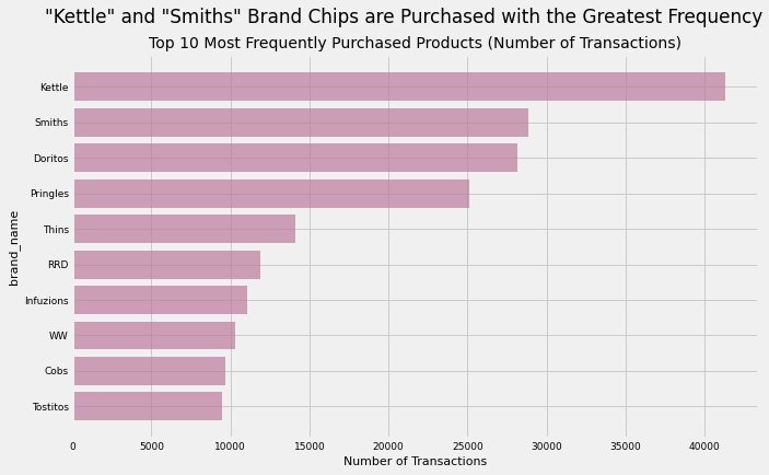
uni_plot('brand_name','#BC7C9C','"Kettle" and "Smiths" Brand Chips are Purchased with the Greatest Frequency','Top 10 Most Frequently Purchased Products (Number of Transactions)')
Takeaways:
Older customers, whether they are married, single, retired or with children purchase chips with the greatest frequency. This suggests these are valuable segments to our client. However, we must note that this is not the same as saying “older customers buy the greatest amount of chip products”. We will explore this particular question later.
The “Kettle” and “Smiths” brands saw the greatest number of purchases by transaction, not by number of chip products sold. “Kettle” chips are a clear outlier because there is a substantial gap between it and 2nd-placed “Smiths” chips. “Pringles” and “Doritos” round out the top 4 with the rest of the pack trailing far behind
6.13) Customer Category
Code
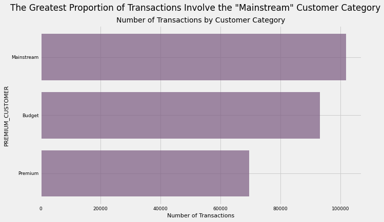
uni_plot('PREMIUM_CUSTOMER','#7A5980','The Greatest Proportion of Transactions Involve the "Mainstream" Customer Category','Number of Transactions by Customer Category')
Takeaways:
Clearly, the greatest number of sales involve the “Mainstream” customer category, while “Premium” customers are responsible for the least number of sales.
However, this is to be expected. Premium customers usually buy higher-priced products and price is inversely correlated with both purchase frequency (as shown here) and purchase quantity.
As a result, while we can say that Mainstream customers purchase chips with the greatest frequency, we cannot say that they are responsible for the greatest revenue for our client. As we have no data on pricing, we are unable to explore this avenue further
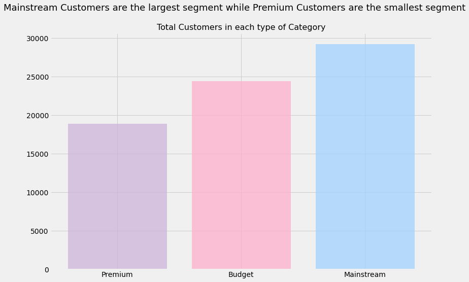
As we did with lifestage, let’s check what proportion of customers belong to each segment
Code
# as we did with lifestage, let's check what proportion of customers belong to each segment
cust_count=[]categories=list(set(merged_df.PREMIUM_CUSTOMER))foriincategories:cust_count.append(merged_df[merged_df['PREMIUM_CUSTOMER']==i]['LYLTY_CARD_NBR'].nunique())cust_per_category=pd.DataFrame({'Category':categories,'num_customers':cust_count})cust_per_category.sort_values(by='num_customers',inplace=True)colors=['#cdb4db','#ffafcc','#a2d2ff']plt.figure(figsize=(12,8))plt.bar(cust_per_category.Category,cust_per_category.num_customers,color=colors,alpha=0.75)plt.title('Total Customers in each type of Category',size=16)plt.suptitle('Mainstream Customers are the largest segment while Premium Customers are the smallest segment',size=18)#plt.tight_layout()
plt.show()
6.14) Evolution of Number of Transactions Through Time
Code
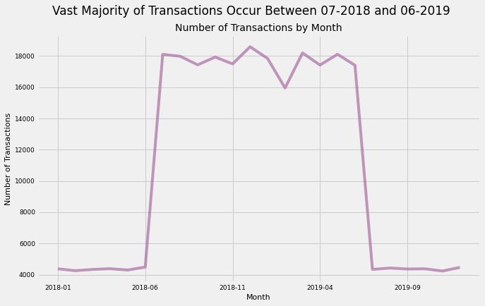
transactions_per_month=merged_df.year_month.value_counts().to_frame()transactions_per_month.reset_index(inplace=True)transactions_per_month.sort_values(by='index',inplace=True)transactions_per_month['index']=transactions_per_month['index'].astype('string')transactions_per_month.plot(x='index',y='year_month',kind='line',figsize=(10,6),color='#A96DA3',alpha=0.7)plt.xlabel('Month',size=11)plt.xticks(size=9)plt.ylabel('Number of Transactions',size=11)plt.yticks(size=9)plt.title('Number of Transactions by Month',size=14)plt.suptitle('Vast Majority of Transactions Occur Between 07-2018 and 06-2019')plt.legend().remove()
Takeaways:
Interestingly, there is a sharp increase in the number of transactions During July 2017. This number stays fairly high and consistent until June 2018, then drops sharply again.
It is not clear from the data why this is occuring. There is no clear seasonality aspect to the sales of chips. Perhaps there was an extremely successful marketing campaign that coincided with this period of high sales, but this is really unlikely.
Whatever factor explains this graph is of paramount importance to the client because it yields an immense increase in sales
6.2) Bivariate Analysis - Total Qty of Products Sold (Best-Selling Products)
6.21) Total Product Sales by Brand - Best-Selling Brand
Code
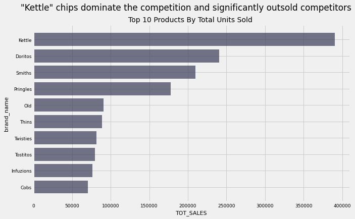
aggregator('brand_name','TOT_SALES','#3B3B58','"Kettle" chips dominate the competition and significantly outsold competitors','Top 10 Products By Total Units Sold ')
Takeaway:
The product with the greatest number of units sold belongs to the “Kettle” and “Doritos” brands. With our previous findings, we can conclude that not only are “Kettle” and “Doritos” brands chips bought most often, they are also bought at the greatest quantities (number of units) overall
For example, “Kettle” chips were bought in over 1 million transactions with almost 4 million units bought. So we can also say that the average number of “Kettle” chips bought per transaction was about 4
As before, “Smiths” and “Pringles” round out the top 4. Interestingly, however, we see that while “Doritos” chips outsold “Smiths” chips in terms of total quantity, Smiths chips were sold more often (by a slight amount). So, on average, customers bought “Smiths” chips more often but in smaller quantities compared to “Doritos” chips
6.22) Total Product Sales by Lifestage
Code
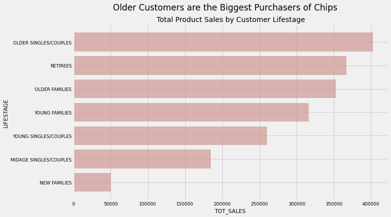
aggregator('LIFESTAGE','TOT_SALES','#CF9893','Older Customers are the Biggest Purchasers of Chips','Total Product Sales by Customer Lifestage')
Takeaway:
We see that not only are Older Singles/Couples, Retirees and Older Families the customer segments that purchase chip products with the greatest frequency, they also purchase the largest quantities of chips.
These findings point to the idea that these segments are very valuable to our client and that the client should continue to target and promote these segments in their supermarket’s strategic plan
6.23) Total Product Sales by Customer Category
Code
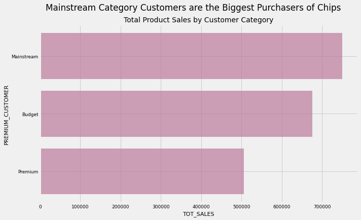
aggregator('PREMIUM_CUSTOMER','TOT_SALES','#BC7C9C','Mainstream Category Customers are the Biggest Purchasers of Chips','Total Product Sales by Customer Category')
Takeaway:
We see a similar distribution here as in the “Customer Category vs Number of Transactions” visualisation.
At first glance, we may think that Mainstream customers are the most valuable to our client because they buy the most products and do so with the greatest frequency. However, this would be an erroneous inference. This is because we have no data on the prices of the products that these customers buy, so we do not know what proportion of total revenue they’re responsible for.
In other words, it is possible (and even likely) that the Premium customers are responsible for the greatest share of revenue for our client. Premium customers have that category name assigned to them for a reason; they likely buy more expensive chips. And finally, it is important to recall that one of the most basic laws of economics states that price is negatively correlated with quantity demanded, so the visualisation above is quite in line with expectations
6.24) Total Product Sales by Packet Size
Code
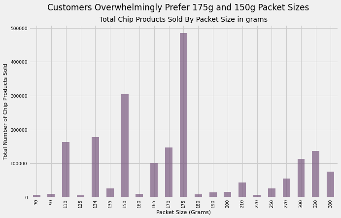
merged_df.groupby('Packet Size')['TOT_SALES'].sum().to_frame().reset_index().plot(kind='bar',x='Packet Size',y='TOT_SALES',figsize=(10,6),color='#7A5980',alpha=0.7)plt.xlabel('Packet Size (Grams)',size=11)plt.ylabel("Total Number of Chip Products Sold",size=11)plt.xticks(size=9)plt.yticks(size=9)plt.title('Total Chip Products Sold By Packet Size in grams',size=14)plt.suptitle('Customers Overwhelmingly Prefer 175g and 150g Packet Sizes')plt.legend().remove()
Takeaway:
175g and 150g, packets that can be considered “medium-sized”, proved to be the most popular with customers.
Interestingly, we see a segment of customers that prefer larger-sized packets as well, ranging from 270g to 380g.
Below we see that for the subset of customers who buy these larger packets, the best-selling brand is “Smiths”, not “Kettle”. Recall that “Kettle” was the best-selling brand overall by a tremendous margin overall, but it is nowhere to be found here. We can conclude that either “Kettle” does not offer large packet sizes or if they do, customers do not prefer larger sizes for this brand
merged_df[merged_df['Packet Size'].isin([270,300,330,380])].groupby('brand_name')['TOT_SALES'].sum().sort_values(ascending=False)# the "Old" value refers to "Old El Palso Salsa Dip". It is not a chips brand so we exclude it
7.2) Most Valuable Segments’ Share of All Product Sales
Code
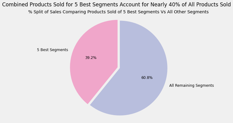
sum_sales_best_segments=sales_best_segments.iloc[:5].sum().sum()labels=['5 Best Segments','All Remaining Segments']sizes=[sum_sales_best_segments,sales_best_segments.TOT_SALES.sum()-sum_sales_best_segments]explode=(0.05,0)colors=['#f0a6ca','#b8bedd']fig1,ax1=plt.subplots(figsize=(6,6))ax1.pie(sizes,explode=explode,labels=labels,autopct='%1.1f%%',shadow=False,startangle=90,textprops={'fontsize':'12'},colors=colors)ax1.axis('equal')plt.title('% Split of Sales Comparing Products Sold of 5 Best Segments Vs All Other Segments',size=14)plt.suptitle('Combined Products Sold for 5 Best Segments Account for Nearly 40% of All Products Sold')#plt.tight_layout()
plt.show()
Takeaway:
The most valuable customer segments, in order, are:
Older Families + Budget
Younger Singles/Couples + Mainstream
Retirees + Mainstream
Young Families + Budget
Older Singles/Couples + Budget
These best segments account for 2 out of every 5 chip products sold, making these extremely valuable segments to target
7.3) Evolution of Spending Patterns Over Time of 5 Best Segments
Code
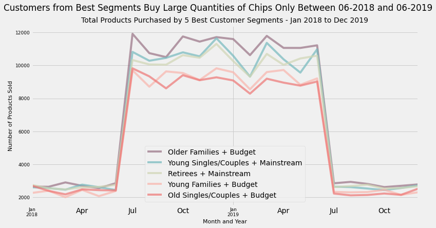
defsegment_sales(lifestage,category,title):df=merged_df.loc[(merged_df['LIFESTAGE']==lifestage)&(merged_df['PREMIUM_CUSTOMER']==category)]df=df.groupby('year_month')['TOT_SALES'].sum().reset_index()df.rename({'TOT_SALES':title},axis=1,inplace=True)returndfolder_fam_budget_sales=segment_sales('OLDER FAMILIES','Budget','old_fam_budget_sales')young_single_mainstream_sales=segment_sales('YOUNG SINGLES/COUPLES','Mainstream','young_single_mainstream_sales')retirees_mainstream_sales=segment_sales('RETIREES','Mainstream','retirees_mainstream_sales')young_families_budget_sales=segment_sales('YOUNG FAMILIES','Budget','youngFam_budget_sales')older_couples_budget_sales=segment_sales('OLDER SINGLES/COUPLES','Budget','old_sin_couple_sales')best_segments_sales=pd.merge(older_fam_budget_sales,young_single_mainstream_sales,on='year_month')best_segments_sales=pd.merge(best_segments_sales,retirees_mainstream_sales,on='year_month')best_segments_sales=pd.merge(best_segments_sales,young_families_budget_sales,on='year_month')best_segments_sales=pd.merge(best_segments_sales,older_couples_budget_sales,on='year_month')best_segments_sales.plot(kind='line',x='year_month',y=['old_fam_budget_sales','young_single_mainstream_sales','retirees_mainstream_sales','youngFam_budget_sales','old_sin_couple_sales'],alpha=0.7,figsize=(12,6),color=['#987284','#75B9BE','#D0D6B5','#F9B5AC','#EE7674'])plt.legend(loc='lower center',labels=['Older Families + Budget','Young Singles/Couples + Mainstream','Retirees + Mainstream','Young Families + Budget','Old Singles/Couples + Budget'])plt.xlabel('Month and Year',size=11)plt.ylabel('Number of Products Sold',size=11)plt.xticks(size=9)plt.yticks(size=9)plt.suptitle('Customers from Best Segments Buy Large Quantities of Chips Only Between 06-2018 and 06-2019')plt.title('Total Products Purchased by 5 Best Customer Segments - Jan 2018 to Dec 2019',size=14)
Takeaway:
Top 3 Best Customer Segments by Number of Products Purchased had fairly similar spending patterns. They all share
A high, sustained level between June 2018 and June 2019 which sees cyclical purchasing behaviour
A dip in that level during February 2019
A peak in that level during March 2019
7.4) Average Frequency of Chip Purchases for Most Valuable Segments
To do this, I can find the difference in number of days for each purchase within a segment then average this.
However, that would introduce a problem: since many different customers can buy chips on a given day, the difference in days between these data points would be 0. This would give a misleading idea of the frequency of chip purchases because the average would be very low due to the nature of the calculations.
To solve this, I need to:
compare the purchase dates of individual (unique) customers within a segment then
compute the average number of days elapsed between purchases for that particular customer then
repeat for a random sample of 1000 customers from that segment
I can then find:
the individual average purchase frequency for each segment (1000 customers each)
the collective average purchase frequency for all 5 segments (5000 customers in total)
Code
# create two lists.
# One to store average number of days elapsed between purchases for each customer
avg_days_purchase_per_cust=[]# One to store the average number of days elapsed between purchases for each segment
avg_days_cust_segment=[]deffreq_purchase(lifestage,category):# filter for required best segment
df=merged_df.loc[(merged_df['LIFESTAGE']==lifestage)&(merged_df['PREMIUM_CUSTOMER']==category)]# randomly sample 1000 customers from this segment
random_cust=list(df.sample(n=1000,random_state=42).LYLTY_CARD_NBR)# write a loop to find the average number of days between purchases for each randomly-sampled customer
foriinrange(len(random_cust)):# isolate to one customer
x=df[df['LYLTY_CARD_NBR']==random_cust[i]].copy()# sort by date
x.sort_values(by=['DATE'],inplace=True)# find difference in days between each purchase
x['Days Since Last Purchase']=(x['DATE']-x['DATE'].shift(1))# fill null values
x['Days Since Last Purchase']=x['Days Since Last Purchase'].fillna(pd.Timedelta(seconds=0))# remove first purchase date because it cannot compare to an 'earlier' date
# then find the mean
avg_1=x.iloc[1:len(df)]['Days Since Last Purchase'].copy().mean()# add each individual customer mean to our pre-defined list list
avg_days_purchase_per_cust.append(avg_1)# when we have collected 1000 customer averages (which comprises a single segment),
# find the average of those 100 averages. This gives the average for the whole segment
# then add this segment-level average to our second pre-defined list
iflen(avg_days_purchase_per_cust)>999:avg_2=pd.to_timedelta(pd.Series(avg_days_purchase_per_cust)).mean()# add average of this segment to another list
avg_days_cust_segment.append(avg_2)# wipe initial list clean for next run of loop
avg_days_purchase_per_cust.clear()else:pass
Code
freq_purchase('OLDER FAMILIES','Budget')freq_purchase('YOUNG SINGLES/COUPLES','Mainstream')freq_purchase('RETIREES','Mainstream')freq_purchase('YOUNG FAMILIES','Budget')freq_purchase('OLDER SINGLES/COUPLES','Budget')avg_days_cust_segment=[x.daysforxinavg_days_cust_segment]avg_days_cust_segment=pd.DataFrame({'Segments':['Older Families + Budget','Younger Singles/Couples + Mainstream','Retirees + Mainstream','Young Families + Budget','Older Singles/Couples + Budget'],'Average Number of Days Between Purchases':avg_days_cust_segment})
Code
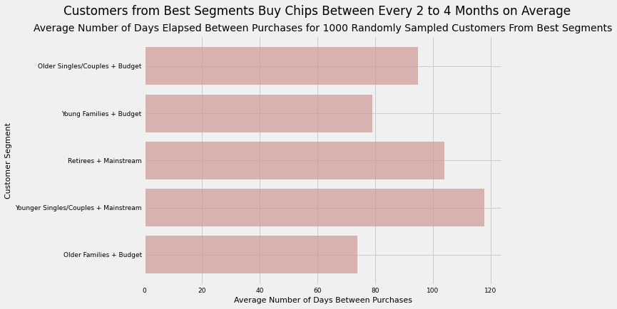
plt.figure(figsize=(8,6))plt.barh(width=avg_days_cust_segment['Average Number of Days Between Purchases'],y=avg_days_cust_segment['Segments'],color='#CF9893',alpha=0.7)plt.xlabel('Average Number of Days Between Purchases',size=11)plt.ylabel('Customer Segment',size=11)plt.xticks(size=9)plt.yticks(size=9)plt.suptitle('Customers from Best Segments Buy Chips Between Every 2 to 4 Months on Average')plt.title('Average Number of Days Elapsed Between Purchases for 1000 Randomly Sampled Customers From Best Segments',size=14)
Takeaways:
Customers from our best segments make purchases on average between every 2 to 4 months.
Among these segments, “Retirees + Mainstream” & “Younger Singles/Couples + Mainstream” are placed near the upper end of this range, with the former in particular taking more than 4 months on average to make a purchase and the latter taking 110 days
The remaining 3 segments all take less than 95 days or just over 3 months to make repeat purchases on average. In particular, “Older Families + Budget” customers take about 75 days to make repeat chips purchases. This segment therefore buys chips with the highest frequency
Interestingly, all of the segments on the lower end of our range come from the “Budget” category. This suggests “Budget” customers are more likely to purchase chips more frequently than either “Mainstream” or “Premium” customers
Segments with “Mainstream” customers are on the upper end of this range
There are no segments with “Premium” customers, further supporting my hypothesis that Premium customers buy fewer products overall with less frequency, but they likely buy the more expensive products
7.5) Average Qty Bought per Customer in Best Segments
Code
print('Average Qty Bought Per Customer in the following segments is: ')print('Older Families + Budget: {:0.2f}'.format(round(older_fam_budget.TOT_SALES.sum()/older_fam_budget.LYLTY_CARD_NBR.nunique()),2))print('Young Singles/Couples + Mainstream: {:0.2f}'.format(young_sing_coup_main.TOT_SALES.sum()/young_sing_coup_main.LYLTY_CARD_NBR.nunique()))print('Retirees + Mainstream: {:0.2f}'.format(retirees_main.TOT_SALES.sum()/retirees_main.LYLTY_CARD_NBR.nunique()))print('Young Families + Budget: {:0.2f}'.format(young_fam_budget.TOT_SALES.sum()/young_fam_budget.LYLTY_CARD_NBR.nunique()))print('Older Singles/Couples + Budget: {:0.2f}'.format(older_sing_coup_budget.TOT_SALES.sum()/older_sing_coup_budget.LYLTY_CARD_NBR.nunique()))
Average Qty Bought Per Customer in the following segments is:
While the Young Singles/Couples + Mainstream and Retirees + Mainstream segments buy more chips overall, they also have a proportionally greater number of customers. This means that, on a per customer basis, the Young Families + Budget segment is more valuable because customers in this segment buy more chips on average than in the two aforementioned segments
8) Conclusions
The “best” segments for our client in the context of their chip-purchasing behaviour when it comes to both frequency and total quantity bought are older customers. In particular, Older Singles/Couples + Budget, Retirees + Mainstream and Older Families + Budget, all of whom also belong to the “Budget” category, all rank near the top of these measures.
However, if we look at the average quantity bought by customers in each segment, then the unifying factor behind the best segments is families and the budget category. This is because Older Families + Budget and Young Families + Budget rank 1st and 2nd in both the frequency of purchasing and in the average qty of chips bought per customer.
Older And Young Families + Budget make a trip to the supermarket to buy chips approximately every 2.5 months, which is by far the greatest frequency. They buy 36 and 34.7 chip products per customer, respectively, over the timeframe of this dataset. Again, this is ranked 1st and 2nd in this measure.
Theoretically, this makes sense. Chips products are usually more popular with children and teens. And of course, if a customer has a family, then they are likely to buy a greater quantity of chips because they may be buying it not only for themselves, but for their family members too.
Along with Young Singles/Couples + Mainstream customers, the aforementioned segments account for 2 out of every 5 units of chips sold.
If we pivot and look at the brand and product-centric inferences, we find that Kettle and Smiths chips dominate the competition by both frequency of purchase and number of units sold. Kettle in particular is a clear outlier here with significant leads over 2nd-placed Smiths in both measures.
Interestingly, when it comes to packet sizes, Kettle does not seem to offer larger packet sizes (those including and above 270g), so Smiths is the most popular brand here. Generally, mid-sized packets (150g, 170g and 175g) are the most popular with customers by far. However, there is a set of customers that does prefer the aforementioned larger packets.
Lastly, there is something peculiar occurring with the purchasing behaviour with respect to time. Something caused total purchases to increase tremendously in June 2018. This stayed at a high level until July 2019, when purchases crashed and returned to pre-June 2019. I am unsure regarding why this occurred. Maybe new supermarkets were opened which increased sales, but that would not explain why sales crashed again in July 2019 (unless these supermarkets were closed in that month). So this warrants further investigation.
Overall, my recommendation to our client is to focus on the segments where customers have families and are in the budget category. Brand-wise, it would be a good idea to promote Kettle, Doritos and Smiths chips overall, and Smiths and Doritos chips in the larger packet sizes
Discover how I used time series-oriented machine learning models to forecast daily sales for Walmart stores, uncovering insights that could reshape retail de...